Past climates· Under the timeline
Climate over the last 350,000 years
350 ka → Today
Under the Sapiens timeline, two colour bands represent how the global mean temperature and the amount of CO₂ (carbon dioxide) in the atmosphere have changed over the last 350,000 years.
The values of the two bands come from measurements since 1850 for the temperature and since 1959 for the CO₂. Before those dates, the temperature comes from published reconstructions, estimates that researchers derive from tree rings, corals, ice and sediments, and the CO₂ from measurements made in air trapped in Antarctic ice.
01What the colours mean
The upper band represents the global mean temperature as a difference from its average over the years 1850-1900. The IPCC, the United Nations panel of climate experts, takes that period as its reference for the climate before industrialisation. A difference of zero corresponds to 13.7 °C, the midpoint of two published estimates, one by Jones and colleagues 1, the other by Rohde and Hausfather 2. The lower band represents the amount of CO₂ in the atmosphere as a ratio to its 1850-1900 level: 1 stands for the same amount, 0.7 for thirty per cent less.
Blues denote a world colder than in 1850-1900, oranges a warmer one, and black, in the middle of the bar, a difference of zero. Near zero, the colours change faster than at the ends of the bar, so that differences of a few tenths of a degree, such as those of the last 2,000 years, remain visible.
On this part of the temperature band, two estimates cover the same dates: one fills the top half, the other the bottom half. From 24,000 to 2,000 years ago, the top half shows the reconstruction of Osman and colleagues 3; the bottom half shows that of Snyder 4 until 12,000 years ago, then that of Kaufman and colleagues 5. The two halves differ by up to 2.3 °C. When the pointer is over the band, or when the band is tapped, a panel opens and displays both values, each with its sources.
In the timeline's colour key, the CO₂ scale is graduated as a ratio to the 1850-1900 level. That level is 289 molecules of CO₂ in every million molecules of air, as measured in air trapped in Antarctic ice 6. The marks and colours of the scale extend from the lowest to the highest CO₂ level in the part of the timeline on screen. The same colour can therefore stand for a different amount from one view to the next; a given temperature, by contrast, always has the same colour.
02Where the values come from
The values used for each part of the bands come from a single study, except where the temperature band is split in two. Where one study takes over from another, the colour can change at once: such a jump is the difference between the two studies, not an abrupt change of climate.
Researchers deduce past temperatures from the growth of tree rings or from the chemistry of shells buried in sediments, which both depend on the temperature of their time. Osman and colleagues 3 combined sea temperatures deduced in this way at scattered sites with a mathematical model of the climate, software that simulates the climate from the laws of physics and extends those temperatures to the whole globe.
| Period | Source | Kind |
|---|---|---|
| 350,000 to 24,000 years ago | Snyder 20164 | reconstruction |
| 24,000 to 12,000 years ago | top halfOsman 20213 | reconstruction |
| bottom halfSnyder 20164 | reconstruction | |
| 12,000 to 2,000 years ago | top halfOsman 20213 | reconstruction |
| bottom halfKaufman 20205 | reconstruction | |
| 1 CE to 1849 | PAGES 2k 20197 | reconstruction |
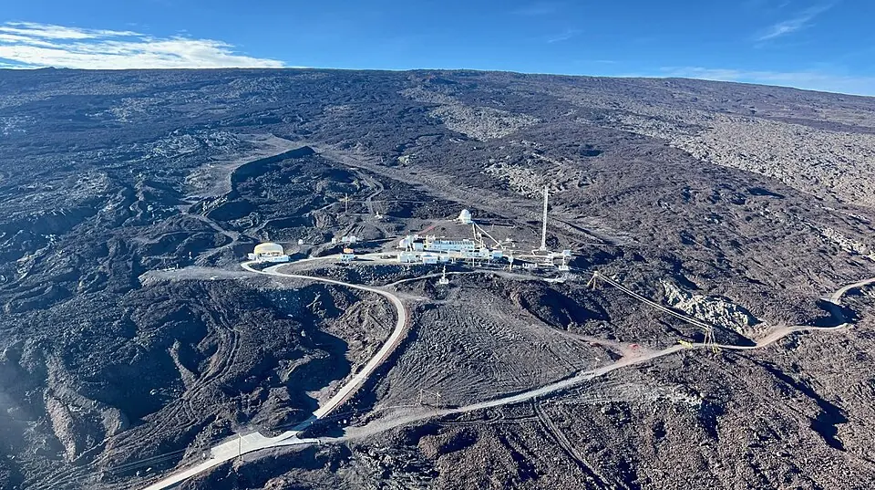
| 1850 to 2025 | Morice 20218 | measurements |
03What the bands do not show
Before 24,000 years ago, the temperature band has only one value per thousand years. It comes from the reconstruction of Snyder 4, built from sea temperatures deduced from marine sediments. Tests on simulated data show that, beyond 40,000 years ago, Snyder's method reliably recovers only changes lasting more than 15,000 years 11. The changes of colour from one thousand years to the next that appear in that part of the band when the timeline is zoomed in are therefore not established changes.
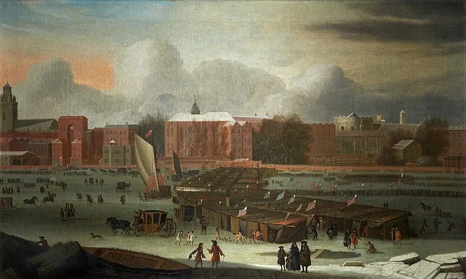
The cooling of about 8,200 years ago, centred on the North Atlantic 12, 13, does not show on the band, which gives the mean temperature of the whole globe. The panel that opens over the band adds an explanation of this kind at seven dates, from the Eemian, the last warm interval before ours, to the eruption of Tambora in 1815.
Under the graduations of the timeline, rows of named bands show the periods of prehistory and, on one of these rows, the climate stages: the cold and temperate periods that geologists distinguish. Most of the boundaries between these stages were set from measurements made on sea-floor sediments at 57 drill sites around the globe 14. On the temperature band, these boundaries fall during a warming or a cooling.